Making sense of Endomondo's calorie estimation [see within blog graph]

The other day I got curious how Endomondo estimates energy expenditure during the exercise.

On their website, they mention some paywalled paper, but no specifics, so I figured it'd be interesting to reverse engineer that myself. My conjecture is that the energy spending should be related to the number of heartbeats during the exercise (since essentialy it's the only objective metric Endomondo gets from me). Let's check how it turns out!

I'm using Wahoo TickrX chest strap monitor, so the HR data coming from it is pretty decent.

First, I'm importing the dataframe from the python package I'm using as the API to interact with my data. I write about it here.

All data is provided by this package, but otherwise it's just a Pandas dataframe:

In [1]:

import my.endomondo
df = my.endomondo.dataframe()

Some sample data:

In [2]:

display(df[df['start_time'].apply(lambda dt: str(dt.date())).isin(['2015-03-06', '2018-05-28', '2020-05-21'])])

	id	start_time	duration	sport	heart_rate_avg	speed_avg	kcal	error
17	481314440	2015-03-06 05:50:38+00:00	0 days 00:52:00	Running	NaN	7.269231	397.0	None
18	481471406	2015-03-06 13:20:06+00:00	0 days 00:30:00	Table tennis	NaN	0.000000	127.0	None
297	1129292141	2018-05-28 10:11:45+00:00	0 days 01:43:10	Cycling	NaN	9.805248	402.0	None
298	1129369900	2018-05-28 12:58:33+00:00	0 days 01:40:14	Cycling	NaN	11.322835	447.0	None
591	1530450975	2020-05-21 08:03:10+00:00	0 days 00:49:54	Running	178.0	12.072150	894.0	None
592	1530492997	2020-05-21 08:56:30+00:00	0 days 00:14:37	Other	114.0	0.000000	121.0	None

Sport type is entered manually when you log the exercise in Endomondo.

Note that I only have HR data for the last few years or so (NaN in heart_rate_avg). For the purposes of this experiment, they need to be filtered out
In addition there is 'Other' type, which doesn't correspond to any sport, it was just me using Endomondo for other HR logging sessions, so it needs to be filtered out
And finally, we need to filter out entries with errors coming from the data provider (the ones that have error value set)

In [3]:

without_hr = df['heart_rate_avg'].isna()
type_other = df['sport'] == 'Other'
without_error = df['error'].notna()
df = df[~(without_hr | type_other | without_error)]

Let's also filter out rare sports that I only did a few times, since they would end up as outliers:

In [4]:

df = df.groupby(['sport']).filter(lambda grp: len(grp) >= 10)

To estimate the number of heartbeats, we can multiply average HR by the duration of the exercise in minutes:

In [5]:

df['heartbeats'] = df['heart_rate_avg'] * df['duration'].dt.total_seconds() / 60

hack to make seaborn plots deterministic (click to expand)

In [6]:

import seaborn as sns
if sns.algorithms.bootstrap.__module__ == 'seaborn.algorithms':
    # prevents nondeterminism in plots https://github.com/mwaskom/seaborn/issues/1924
    # we only want to do it once
    def bootstrap_hacked(*args, bootstrap_orig = sns.algorithms.bootstrap, **kwargs):
        kwargs['seed'] = 0
        return bootstrap_orig(*args, **kwargs)
    
    sns.algorithms.bootstrap = bootstrap_hacked

In [7]:

%matplotlib inline
import matplotlib
import matplotlib.pyplot as plt
plt.style.use('seaborn')
import seaborn as sns
sns.set(font_scale=1.5)

sports = {
    g: len(f) for g, f in df.groupby(['sport'])
}

g = sns.lmplot(
    data=df,
    x='heartbeats',
    y='kcal',
    hue='sport', 
    hue_order=sports.keys(),
    legend_out=False,
    height=15,
    palette='colorblind',
    truncate=False, # kind of sets same span for the reglines
)
ax = g.ax
ax.set_title('Dependency of energy spent during exercise on number of heartbeats')

ax.set_xlim((0, None))
ax.set_xlabel('Total heartbeats, measured by chest strap HR monitor')

ax.set_ylim((0, None))
ax.set_ylabel('Kcal,\nEndomondo\nestimate', rotation=0, y=1.0)

# https://stackoverflow.com/a/55108651/706389
plt.legend(
    title='Sport',
    labels=[f'{s} ({cnt} points)' for s, cnt in sports.items()],
    loc='upper left',
)
pass

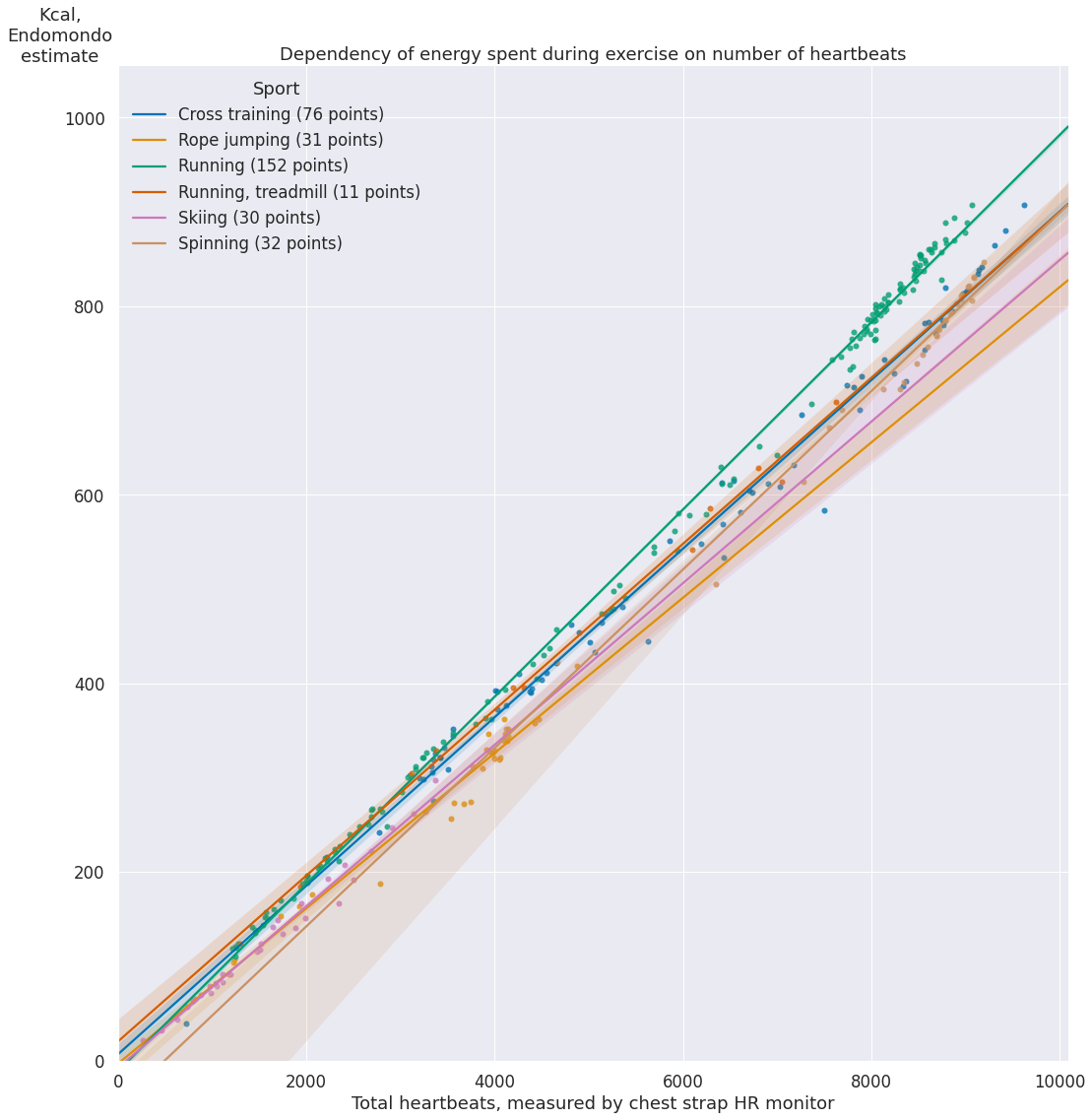
Unsurprisingly, it looks like a simple linear model (considering my weight and age have barely changed).

What I find unexpected is that the slope/regression coefficient (i.e. calories burnt per heartbeat) is more or less the same. Personally, for me running feels way more intense than any of other cardio I'm doing, definitely way harder than skiing! There are two possibilities here:

Endomondo can't capture dynamic muscle activity and isn't even trying to use exercise type provided by the user for a better estimate.
Energy is mostly burnt by the heart and other muscles don't actually matter or have a very minor impact.

Let's try and check the latter via some back of an envelope calculation.

In order to run, you use your chemical energy to move your body up and forward. For simplicity, let's only consider 'up' movements that go against gravity, it feels like these would dominate energy spendings. So let's model running as a sequence of vertical jumps. My estimate would be that when you run you jumps are about 5 cm in height.

We can find out how much energy each jump takes by using $\Delta U = m g \Delta h$ formula.

In [8]:

g = 9.82 # standard Earth gravity
weight = 65 # kg
stride_height = 5 / 100 # convert cm to m

strides_per_minute = 160 # ish, varies for different people
duration = 60 # minutes
joules_in_kcal = 4184 

energy_per_stride = weight * g * stride_height

leg_energy_kcal = energy_per_stride *  strides_per_minute * duration / joules_in_kcal
print(leg_energy_kcal)

73.22753346080309

So, 70 kcal is fairly low in comparison with typical numbers Endomondo reports for my exercise.

This is a very rough calculation of course:

In reality movements during running are more complex, so it could be an underestimate
On the other hand, feet can also spring, so not all energy spent on the stride is lost completely, so it could be an overestimate

With regards to the actual value of the regression coefficient: seaborn wouldn't let you display them on the regplot, so we use sklearn to do that for us:

In [9]:

from sklearn import linear_model

reg = linear_model.LinearRegression()
reg.fit(df[['heartbeats']], df['kcal'])

[coef] = reg.coef_
intc = reg.intercept_

print(f"Regression coefficient: {coef:.3f}")
print(f"Intercept: {intc:.3f}")

Regression coefficient: 0.096
Intercept: -17.057

Basically, that means I get about 0.1 Kcal for each heartbeat during exercise. The intercept should ideally be equal to 0 (i.e. just as a sanity sort of thing: not having heartbeat shouldn't result in calorie loss), but what we have is close enough.

Also, fun calculation: what if we fit the model we got to normal, resting heart rate?

In [10]:

normal_bpm = 60
minutes_in_day = 24 * 60

print(f'{coef * normal_bpm * minutes_in_day:.3f}')

8296.861

8K Kcals per day? A bit too much for an average person. I wouldn't draw any conclusions from that one though :)

You can find the source of this notebook here.

Discussion:

/r/dataisbeautiful