Analyzing accuracy of power reported by stationary bike [see within blog graph]

How I found my exercise machine to violate laws of physics

I was curious how effort exerted during the exercise impacts heart rate and whether that correlates strongly with subjective fatigue and exhaustion.

It seemed that easiest way to experiment would be stationary bike. Running only has single variable, speed. One could of course change incline, but that would be harder to predict.

For elliptical machine or rowing machine it would be even more complicated!

With stationary bike, there are two variables that potentially impact power you need to exert:

RPM (revolutions per minute), or angular velocity, that should have linear effect on power (no air resistance as it's stationary!)
resistance, which isn't exactly specified, but one would expect it to be proportional to the force you have to apply (i.e. torque)

Or, simply put, $P = \tau \omega$ (wiki )

The indoor exercise bike displays the pace (i.e. revolutions per minute), so all you have to do is maintain it. In addition it's displaying current resistance level (you can set it by adjusting a mechanical knob) and reports power in watts.

During exercise, I'm using a chest HR tracker, so simplest thing to do would be take whatever power the machine reports and try to find correlation with moving total/average of HR.

However, being paranoid and lacking any documentation for the machine, I decided no to trust its numbers blindly and check them instead. Technogym's website doesn't help in clarifying how power is computed. They have some sensible information like:

The power meter must be accurate.

The power measurement must be precise and repeatable. A 3-5 watt error is not significant, but if a system is not reliable there may be deviations of many tens of watts, i.e. equal to or greater than the amount of power that is gained from one year's training.

Let's see how accurate is their power meter!

Initial measurements (2019-11-09)¶

Throughout different exercise sessions, I've taken bunch of measurements of RPM, resistance and power:

Measurements (click to expand)

In [1]:

# TODO could only collapse inputs?
datas = """
58 10 129
56 10 127
56 10 127
56 8  94
57 8  98
56 8  94
58 10 133
56 10 126
56 8  93
55 8  91
56 8  94
56 10 128
55 10 124
54 10 119
53 8  87
55 8  93
55 8  90
95 8  240

70 10 198
55 8  85
95 8  226
95 8  229
95 8  228
95 8  227

97 8  236
95 8  227
95 8  227
95 8  230
60 10 156
61 10 154
62 10 162
61 10 156
55 10 125
56 10 128
57 8  89
56 8  87
57 8  90
57 8  91
60 8  101
56 10 129
57 10 131
"""

import pandas as pd
def make_df(datas: str) -> pd.DataFrame:
    df = pd.DataFrame(
        (map(int, l.split()) for l in datas.splitlines() if len(l.strip()) > 0),
        columns=['rpm', 'resistance', 'watts'],
    )
    df.index = df.apply(lambda row: f"{row['rpm']}_{row['resistance']}_{row['watts']}", axis='columns')
    return df

df = make_df(datas)
old_df = df.copy()
# btw, if anyone knows a more elegant way of converting such a table in dataframe, I'd be happy to know!

In [2]:

display(df.sample(10, random_state=0))

	rpm	resistance	watts
95_8_227	95	8	227
56_8_87	56	8	87
61_10_154	61	10	154
57_8_98	57	8	98
56_8_94	56	8	94
61_10_156	61	10	156
95_8_230	95	8	230
56_10_128	56	10	128
57_8_90	57	8	90
62_10_162	62	10	162

It's reasonable to assume that power depends linearly both on RPM and resistance, so we conjecture watts = rpm x resistance. Let's see if it holds against what the exercise bike reports:

hack to make seaborn plots deterministic (click to expand)

In [3]:

import seaborn as sns
if sns.algorithms.bootstrap.__module__ == 'seaborn.algorithms':
    # prevents nondeterminism in plots https://github.com/mwaskom/seaborn/issues/1924
    # we only want to do it once
    def bootstrap_hacked(*args, bootstrap_orig = sns.algorithms.bootstrap, **kwargs):
        kwargs['seed'] = 0
        return bootstrap_orig(*args, **kwargs)
    
    sns.algorithms.bootstrap = bootstrap_hacked
    
# apparently because of a dependency    
# https://github.com/statsmodels/statsmodels/blob/fdd61859568c4863de9b084cb9f84512be55ab33/setup.cfg#L17
import warnings
warnings.filterwarnings('ignore', 'Method .ptp is deprecated and will be removed.*', FutureWarning, module='numpy.*')

In [4]:

%matplotlib inline
import matplotlib
from matplotlib import pyplot as plt
plt.style.use('seaborn')
import seaborn as sns
sns.set(font_scale=1.25) # TODO not sure?

def plot_df(df):
    dff = df.copy()
    dff['rpm x resistance'] = df['rpm'] * df['resistance']
    if 'color' not in dff:
        dff['color'] = 'blue'

    fig, ax = plt.subplots(figsize=(10, 10))
    plt.xlim((0, max(dff['rpm x resistance']) * 1.1))
    plt.ylim((0, max(dff['watts']) * 1.1))

    g = sns.regplot(
        data=dff,
        x='rpm x resistance', y='watts',
        ax=ax,
        scatter_kws={'facecolors':dff['color']},
        truncate=False,
    )

    plt.xlabel('Power, theoretical, angular velocity multiplied by resistance')
    plt.ylabel('Power, watts as reported by the machine')

    plt.show()

plot_df(df)

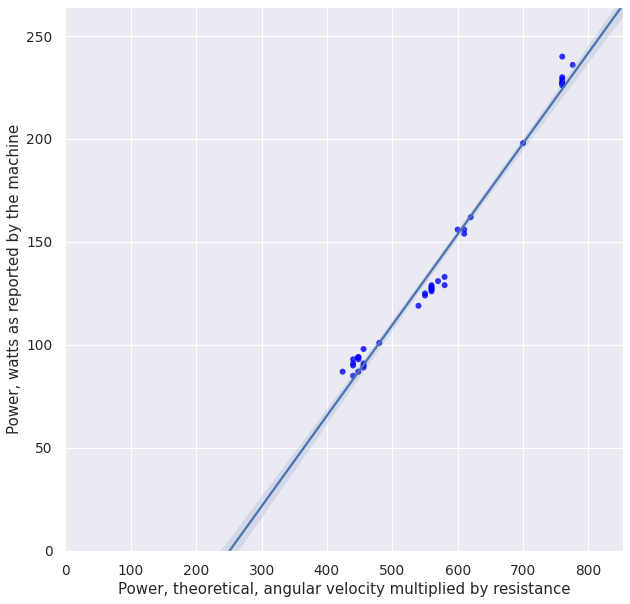
Wow, that doesn't look so well, I'd expect the regression line to intersect (0, 0). Let's double check this:

In [5]:

import statsmodels.api as sm
def print_stats(df):
    dff = df.copy()
    dff['rpm x resistance'] = df['rpm'] * df['resistance']
    X = dff[['rpm x resistance']]
    X = sm.add_constant(X)
    res = sm.OLS(dff['watts'], X).fit()
    summary = str(res.summary())
    import re # filter out nondeterministic stuff from the report
    summary = re.sub('Date:.*\d{4}.*\n', '', str(summary))
    summary = re.sub('Time:.*\d{2}:\d{2}:\d{2}.*\n', '', str(summary))
    print(summary)
print_stats(df)

                            OLS Regression Results                            
==============================================================================
Dep. Variable:                  watts   R-squared:                       0.982
Model:                            OLS   Adj. R-squared:                  0.981
Method:                 Least Squares   F-statistic:                     2109.
No. Observations:                  41   AIC:                             281.4
Df Residuals:                      39   BIC:                             284.8
Df Model:                           1                                         
Covariance Type:            nonrobust                                         
====================================================================================
                       coef    std err          t      P>|t|      [0.025      0.975]
------------------------------------------------------------------------------------
const             -110.6016      5.605    -19.732      0.000    -121.939     -99.264
rpm x resistance     0.4406      0.010     45.929      0.000       0.421       0.460
==============================================================================
Omnibus:                        1.196   Durbin-Watson:                   1.017
Prob(Omnibus):                  0.550   Jarque-Bera (JB):                1.049
Skew:                          -0.190   Prob(JB):                        0.592
Kurtosis:                       2.315   Cond. No.                     2.87e+03
==============================================================================

Notes:
[1] Standard Errors assume that the covariance matrix of the errors is correctly specified.
[2] The condition number is large, 2.87e+03. This might indicate that there are
strong multicollinearity or other numerical problems.

Free parameter is about -100 watts, which is quite a lot considering my high intensity intervals are 250 watts (so it means about 40% error!). I don't think it can be explained by friction either: if anything, friction would shift the plot up and make the free coefficient positive.

At this point, I'm not sure what it means. I guess I'll try to make more measurements at really low resistances and speeds to make the model more complete, but I would be too surprised if either watts or resistance reported by the machine are just made up.

More data (2019-11-14)¶

I collected more data corresponding to different resistances/velocities. It's actually quite hard to consistently spin under low resistance setting, so I think I might need one more round of data collection to complete the picture!

More measurements (click to expand)

In [6]:

new_df = make_df("""
96  4  66
99  4  69
101 6  146
103 6  149
110 6  166
111 6  170
50  13 186
36  13 107
36  13 105
31  10 41
30  10 44
28  10 39
117 8  323
116 8  320
116 8  322
48  6  40
49  6  37
60  2  24
59  2  23
86  2  40
106 2  48
62  5  44
61  5  44
81  5  70
81  5  70
93  5  90
97  5  97
35  12 87
33  12 81
25  12 51
26  12 55
27  1  50
39  8  46
39  8  44
30  8  29
30  8  31
32  8  31
32  8  31
29  8  29
""")

In [7]:

df = pd.concat([old_df, new_df])
plot_df(df)
print_stats(df)

                            OLS Regression Results                            
==============================================================================
Dep. Variable:                  watts   R-squared:                       0.924
Model:                            OLS   Adj. R-squared:                  0.923
Method:                 Least Squares   F-statistic:                     952.2
No. Observations:                  80   AIC:                             709.6
Df Residuals:                      78   BIC:                             714.3
Df Model:                           1                                         
Covariance Type:            nonrobust                                         
====================================================================================
                       coef    std err          t      P>|t|      [0.025      0.975]
------------------------------------------------------------------------------------
const              -60.3329      6.129     -9.843      0.000     -72.535     -48.130
rpm x resistance     0.3614      0.012     30.857      0.000       0.338       0.385
==============================================================================
Omnibus:                       57.648   Durbin-Watson:                   1.094
Prob(Omnibus):                  0.000   Jarque-Bera (JB):              238.330
Skew:                           2.326   Prob(JB):                     1.77e-52
Kurtosis:                      10.062   Cond. No.                     1.42e+03
==============================================================================

Notes:
[1] Standard Errors assume that the covariance matrix of the errors is correctly specified.
[2] The condition number is large, 1.42e+03. This might indicate that there are
strong multicollinearity or other numerical problems.

Ok, it clearly started diverging from the nice linear dependency, especially at lower values of theoretical power. It's time to try to break it down and see what is to blame: e.g., resistance or speed component, or perhaps some individual measurements.

Analyzing data and looking at outliers (2019-11-24)¶

In [8]:

import statsmodels.api as sm
def plot_influence(df):
    # TODO FIXME use it in prev section
    res = sm.formula.ols("watts ~ rpm * resistance - resistance - rpm", data=df).fit()
    fig, ax = plt.subplots(figsize=(10, 10))
    sm.graphics.influence_plot(res, ax=ax, criterion="cooks")
    plt.show()
plot_influence(df)
# sm.graphics.plot_partregress_grid(res, fig=fig)

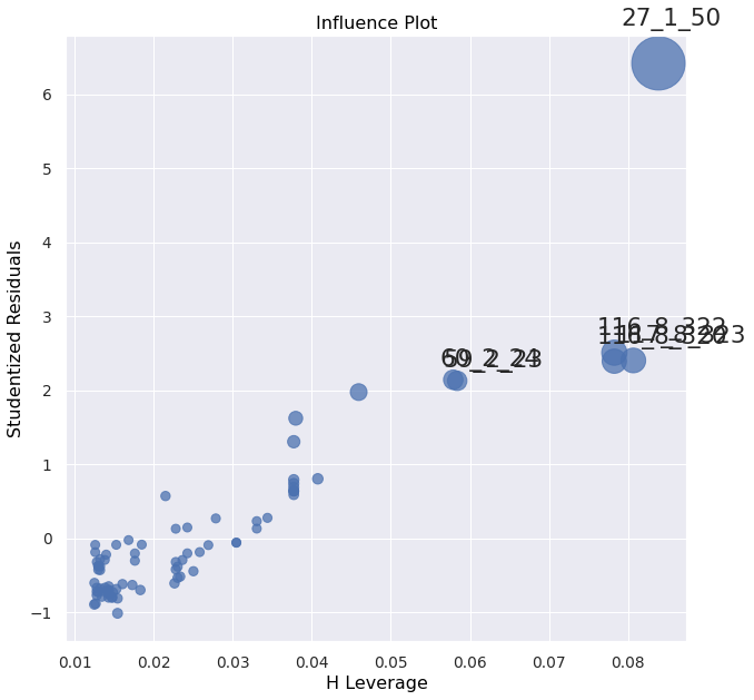
TODO hmm, 0.10 is not that high leverage right? Although depends on residual too, and here the residual is very high, so it would have high influence.. https://www.statsmodels.org/dev/examples/notebooks/generated/regression_plots.html

'27_1_50' seems like a typo. Let's drop it and ignore.

In [9]:

fdf = df.drop([
    '27_1_50',
])

Ok, that's somewhat better at least in terms of outliers. Let's see if that helps:

In [10]:

plot_df(fdf)
print_stats(fdf)

                            OLS Regression Results                            
==============================================================================
Dep. Variable:                  watts   R-squared:                       0.950
Model:                            OLS   Adj. R-squared:                  0.949
Method:                 Least Squares   F-statistic:                     1467.
No. Observations:                  79   AIC:                             667.9
Df Residuals:                      77   BIC:                             672.7
Df Model:                           1                                         
Covariance Type:            nonrobust                                         
====================================================================================
                       coef    std err          t      P>|t|      [0.025      0.975]
------------------------------------------------------------------------------------
const              -69.9960      5.203    -13.454      0.000     -80.356     -59.636
rpm x resistance     0.3784      0.010     38.307      0.000       0.359       0.398
==============================================================================
Omnibus:                       27.329   Durbin-Watson:                   0.562
Prob(Omnibus):                  0.000   Jarque-Bera (JB):               40.545
Skew:                           1.500   Prob(JB):                     1.57e-09
Kurtosis:                       4.823   Cond. No.                     1.49e+03
==============================================================================

Notes:
[1] Standard Errors assume that the covariance matrix of the errors is correctly specified.
[2] The condition number is large, 1.49e+03. This might indicate that there are
strong multicollinearity or other numerical problems.

So, on one hand that did make fit look more linear. On the other hand we've had to filter out all the low-resistance observations to achieve that.

I guess I'll collect more observations to be absolutely sure.

TODO add TOC or something?

Even more data (2019-11-25)¶

I've collected a bit more data, especially at lower velocities and resistance:

More measurements (click to expand)

In [11]:

new_df_2 = make_df("""
113 2  50
73  2  32
71  2  30
70  2  29
107 3  64
108 3  65
114 4  103
48  4  25
40  4  20
31  13 81
36  16 163
40  5  24
35  6  23
31  7  23
31  9  40
40  9  64
115 6  175
109 6  163
31  12 72
30  13 76
54  4  33
38  4  19
75  4  55
36  8  40
39  8  46
32  8  34
70  3  39
49  3  22
37  3  14
""")

ndf = pd.concat([fdf, new_df_2])

Let's check for outliers first:

In [12]:

plot_influence(ndf)

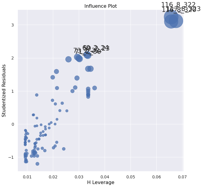
Residuals of 3 are borderline, but don't immediately mean outliers.

Let's plot and analyze! Just out of curiosity, in addition we'll color values corresponding to different resistances (the darker, the more resistance):

In [13]:

ress = list(sorted(set(ndf['resistance'])))
colors = dict(zip(ress, sns.light_palette('navy', n_colors=len(ress))))
ndf['color'] = [colors[x] for x in ndf['resistance']]
# if you know of an easier way to use column value as a color in seaborn, please let me know!
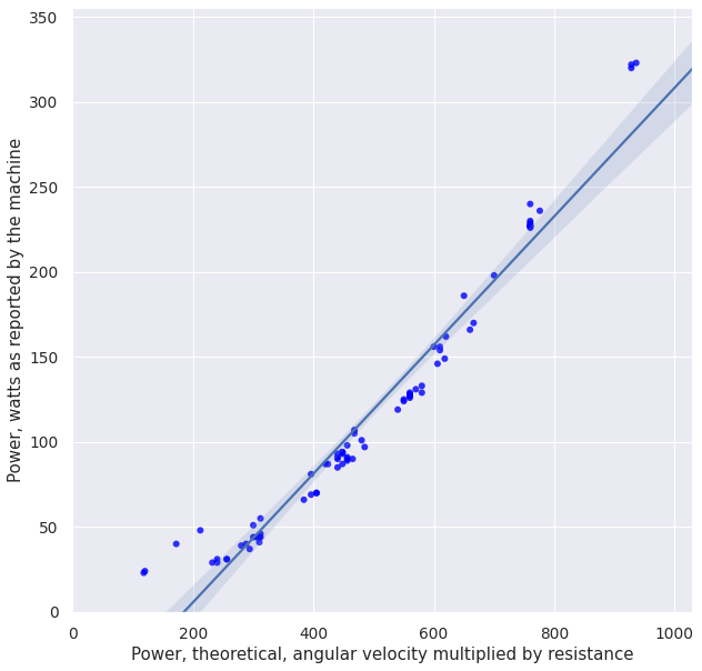
plot_df(ndf)
print_stats(ndf)

                            OLS Regression Results                            
==============================================================================
Dep. Variable:                  watts   R-squared:                       0.943
Model:                            OLS   Adj. R-squared:                  0.942
Method:                 Least Squares   F-statistic:                     1754.
No. Observations:                 108   AIC:                             922.1
Df Residuals:                     106   BIC:                             927.5
Df Model:                           1                                         
Covariance Type:            nonrobust                                         
====================================================================================
                       coef    std err          t      P>|t|      [0.025      0.975]
------------------------------------------------------------------------------------
const              -52.5400      4.002    -13.130      0.000     -60.474     -44.606
rpm x resistance     0.3483      0.008     41.880      0.000       0.332       0.365
==============================================================================
Omnibus:                       20.686   Durbin-Watson:                   0.646
Prob(Omnibus):                  0.000   Jarque-Bera (JB):               25.653
Skew:                           1.159   Prob(JB):                     2.69e-06
Kurtosis:                       3.574   Cond. No.                     1.17e+03
==============================================================================

Notes:
[1] Standard Errors assume that the covariance matrix of the errors is correctly specified.
[2] The condition number is large, 1.17e+03. This might indicate that there are
strong multicollinearity or other numerical problems.

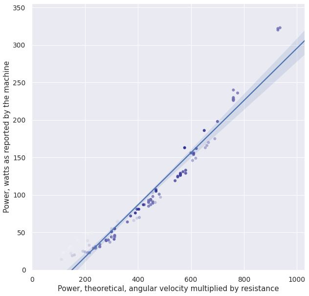
So, there is a clear trend of points clumping towards 0, which means that the model ceases to be linear.

If we try to fit the line to the points in a more reasonable exercise range (e.g. at least 50 RPM and resistance of 6, which would mean Power >= 300), that would skew the regression line even more to the right and move the coefficient even further away from zero.

So overall it means that either:

the assumption of linear dependency on resistance and velocity is wrong, but then it's completely unclear how the power is estimated
I wasn't accurate during measurements on lower intensities, but I think it's pretty unlikely as I did multiple measurement sessions and even if you ignore the higher variance, mean is still way above the regression line
the velocity/resistance reported by the machine are wrong or misleading. It's possible that the number machine assigns to 'resistance' doesn't really mean anything.

Conclusion¶

¯\(ツ)/¯

I guess be careful about trusting the equipment and do your own experiments.

As you can see, my initial project of finding some correlation with my HR turned out in a completely different direction.

Next steps¶

Would be interesting to at least compare watts (theoretical and reported by the machine) versus calories estimated by Endomondo (which takes heart rate into account).