THIS IS A DRAFT! It will appear on the main page once finished!

They see me flowin' they hatin'

Some questionable experiments with Lagrangians

A while ago when I was learning classical mechanics I started wondering what makes a good physical Lagrangian and how does its shape impact the laws of motion. I seem to be more of software engineer than a physycist in spirit so rather than learning classical mechanics, instead I ended up doing various experiments with plotting, rendering, modelling and literate programming. So while I'm not exactly doing any novel physics here, I also haven't seen this visualised anywhere (apart from the simplest case). Hopefully it will help other people in understanding and serve as a demo of Ipython's capabilities.

This post assumes some basic (wikipedia level TODO link?) understanding of Lagrangian/Hamiltonian mechanics, but you don't have to if you just fancy some plots. For the purposes of this post, Lagrangian is just any function of a particle's position and velocity.

Routines for easier multiline printing (click to expand)

In [1]:

# see https://beepb00p.xyz/ipynb-singleline.html

def ldisplay_md(fmt, *args, **kwargs):
    from IPython.display import Markdown
    display(Markdown(fmt.format(
        *(f'${latex(x)}$' for x in args),
        **{k: f'${latex(v)}$' for k, v in kwargs.items()})
    ))
    
def as_text(thing):
    from IPython.core.interactiveshell import InteractiveShell # type: ignore
    plain_formatter = InteractiveShell.instance().display_formatter.formatters['text/plain']
    pp = plain_formatter(thing)
    lines = pp.splitlines()
    return lines

def vcpad(lines, height):
    width = len(lines[0])
    missing = height - len(lines)
    above = missing // 2
    below = missing - above
    return [' ' * width for _ in range(above)] + lines + [' ' * width for _ in range(below)]

# terminal and emacs can't display markdown, so we have to use that as a workaround
def mdisplay_plain(fmt, *args, **kwargs):
    import re
    from itertools import chain
    fargs   = [as_text(a) for a in args]
    fkwargs = {k: as_text(v) for k, v in kwargs.items()}

    height = max(len(x) for x in chain(fargs, fkwargs.values()))

    pargs   = [vcpad(a, height) for a in fargs]
    pkwargs = {k: vcpad(v, height) for k, v in fkwargs.items()}

    textpos = height // 2

    lines = []
    for h in range(height):
        largs   = [a[h] for a in pargs]
        lkwargs = {k: v[h] for k, v in pkwargs.items()}
        if h == textpos:
            fstr = fmt
        else:
            # we want to keep the formatting specifiers (stuff in curly braces and empty everything else)
            fstr = ""
            for e in re.finditer(r'{.*?}', fmt):
                fstr = fstr + " " * (e.start() - len(fstr))
                fstr += e.group()
        lines.append(fstr.format(*largs, **lkwargs))
    for line in lines:
        print(line.rstrip())

ldisplay = ldisplay_md

In [2]:

%matplotlib inline
from sympy import *
from sympy import diff as D, Function as F

t = symbols('t', real=True) # time
q = F('q')(t) # position
v = F('v')(t) # velocity
p = F('p')(t) # [conjugate] momentum

Sadly, jupyter's capabilities for literate programing turned out to be poorer than I expected... Basically, you can't split a function among several cells. (TODO perhaps hack it via CSS or something?) So, over the course of the following function I'm gonna communicate with you via comments.

In [3]:

def lagrangian_to_hamiltons_equations(Lag): # So, we've got a Lagrangian: ldisplay("$L$ = {}", Lag) """ To actually get the laws of motion it's way more convenient to solve Hamilton's equations. It's fairly easy to get them via something called Legendre transormation: https://en.wikipedia.org/wiki/Hamiltonian_mechanics#Calculating_a_Hamiltonian_from_a_Lagrangian """ p_of_v = Eq(p, Lag.diff(v)) [sol] = solve(p_of_v, v) v_of_p = Eq(v, sol) ldisplay("$p$ over $v$: {}", p_of_v) ldisplay("$v$ over $p$: {}", v_of_p) # looks like variable replacement in Sympy is a bit more tedious than I expected H = (v * p_of_v.rhs - Lag).subs({v_of_p.lhs: v_of_p.rhs}) ldisplay("$H$ = {}", H) # cool, we've got Hamiltonian dq_eq = Eq(q.diff(t), H.diff(p)) dp_eq = Eq(p.diff(t), -H.diff(q)) ldisplay("Hamilton's equations: {}", [dq_eq, dp_eq]) from sympy.solvers.ode.ode import classify_sysode print(classify_sysode([dq_eq, dp_eq])) """ lambdify is neat! It substitutes numpy equivalents for sympy functions, so we get decent performance. """ dq = lambdify((q, p, t), dq_eq.rhs) dp = lambdify((q, p, t), dp_eq.rhs) """ Ok, let's finally have a break from this function, the actual numerical solving can be extracted in a different function """ return (dq, dp)

Ok, now we need to define some slightly cryptic routines to integrate and plot stuff. Hopefully, later their purpose would become more clear.

In [4]:

import functools
class Lagrangian:
    """
    This class represents both symbolic Lagrangian for plotting convenience and
    also caches computations for Hamilton's equations
    """
    def __init__(self, expr):
        self.lag = expr
        
    @property
    @functools.lru_cache(1)
    def dq_dp(self):
        return lagrangian_to_hamiltons_equations(self.lag)

Routines for integration and plotting (click to expand)

In [5]:

import matplotlib.pyplot as plt
plt.rcParams['figure.figsize'] = [9, 9]
from sympy.plotting import plot, plot_parametric
from scipy.integrate import odeint 
import numpy as np
from numpy import linspace

def plot_motion(
    lagrangian, 
    q0p0s=[], # initial data
    T_max=20, T_steps=1000, 
    q_max=None, 
    p_max=None,
    plot_lag=True,
    plot_pq=True,
    plot_phase=True,
    plot_legends=True,
):
    dq, dp = lagrangian.dq_dp
    
    N = len(q0p0s)
    labels = [f'{float(qq):.1f}, {float(pp):.1f}' for (qq, pp) in q0p0s]
    
    times = linspace(0, T_max, T_steps)
    def integrate_step(qp, t):
        prev_q, prev_p = qp
        next_q = dq(prev_q, prev_p, t)
        next_p =  dp(prev_q, prev_p, t)
        return (next_q, next_p)
    
    all_ts = []
    all_qs = []
    all_ps = []
    for q0, p0 in q0p0s:
        sol = odeint(integrate_step, (q0, p0), times)
        all_ts.append(times)
        all_qs.append(sol[:, 0])
        all_ps.append(sol[:, 1])

    # ok, let's plot everything now!

    blues  = plt.cm.winter(linspace(0, 1, N))
    reds   = plt.cm.autumn(linspace(0, 1, N))
    greens = plt.cm.Set1(linspace(0.5, 1, N))
    
    # TODO display trajectories on Lagrangian?
    # TODO also make a note that it's not easy to see how would the trajectory make action stationary
    if plot_lag:
        from mpl_toolkits.mplot3d import Axes3D
        plt.figure(figsize=(12, 12)) # TODO how to configure it?
        step = 0.1 # TODO ?
        x = np.arange(-q_max, q_max, step)
        y = np.arange(-p_max, p_max, step)
        X, Y = np.meshgrid(x, y)
        Z = lambdify((q, v), lagrangian.lag)(X, Y)
        ax3d = plt.subplot(111, projection='3d')
        ax3d.set_title(f'Lagrangian {lagrangian.lag}')
        ax3d.set_xlabel('q')
        ax3d.set_ylabel('v')
        ax3d.set_zlabel('L')
        ax3d.plot_surface(X, Y, Z)
        plt.show()    
        
    if plot_pq:
        plt.figure(figsize=(7,7))
        plt.grid()
        plt.title('position/momentum over time')
        plt.xlabel('t')
        plt.ylabel('q,p')
        for label, ts, qs, ps, blue, red in zip(labels, all_ts, all_qs, all_ps, blues, reds):
            plt.plot(ts, qs, color=blue, label=f'q {label}')
            plt.plot(ts, ps, color=red, label=f'p {label}')
        if plot_legends: plt.legend(loc='upper left')
        plt.show()

    if plot_phase:
        plt.figure(figsize=(15,7))
        from mpl_toolkits.mplot3d import Axes3D
        ax = plt.subplot(1, 2, 1)
        ax3d = plt.subplot(1, 2, 2, projection='3d')
    
        ax.grid()
        ax.set_title('phase plot')
        ax.set_xlabel('q(t)')
        ax.set_ylabel('p(t)')
        if q_max is not None: ax.set_xlim((-q_max, q_max))
        if p_max is not None: ax.set_ylim((-p_max, p_max))
        for label, ts, qs, ps, green in zip(labels, all_ts, all_qs, all_ps, greens):
            ax.plot(qs, ps, color=green, label=f'{label}')
        if plot_legends: ax.legend(loc='upper left')

        ax3d.grid()
        ax3d.set_title('phase plot')
        ax3d.set_xlabel('q')
        ax3d.set_ylabel('p')
        ax3d.set_zlabel('t')
        if q_max is not None: ax3d.set_xlim((-q_max, q_max))
        if p_max is not None: ax3d.set_ylim((-p_max, p_max))
        for label, ts, qs, ps, green in zip(labels, all_ts, all_qs, all_ps, greens):
            ax3d.plot(qs, ps, ts, color=green, label=label)
        if plot_legends: ax3d.legend(loc='upper left')
        plt.show()

Ok, now that we defined the boilerplate, we're ready actually do something.

(TODO heading and TOC?)

The first test subject is the default textbook choice: the harmonic oscillator. It's a familiar system to many and a good warmup.

In [6]:

# TODO plot lagrangian first?
# then try to meditate if we can spot stationary trajectories
# one obvious choice is (0, 0), the saddle point. it would correspond to the pendulum staying still, and indeed a feasible physical trajectory
# 
# TODO ok, so maybe plot solutions on the lagrangian first? (e.g. just say we took them from wikipedia)
# and then experiment if one can tell them from non-solutions

# NOTE: I deliberately pick different magnitudes, because otherwise plots would overlap
# TODO if it was interactive, could try by themselves?
L_harm = Lagrangian(v ** 2 / 2 - q ** 2 / 2)
# NOTE: while 1/2 is not necessary, it does result in somewhat cleaner numeric results
# TODO show time on phase plots?
plot_motion(
    L_harm, 
    q0p0s=[
        (-4, 4),
        (5 , 5),
        (6 , -6),
        (-7, -7),
    ],
    q_max=10,
    p_max=10,
)
# TODO don't like the 'p over v' text? rephrase?
# TODO plot trajectories on the lagrangian?
# NOTE: I don't know about you, but I certainly can't easily tell from the way the trajectory looks whether it's stationary or not
# TODO try different coordinates

# TODO actually, non-uniqueness of the Lagrangian problem could be demonstrated by taking q_1, q_2 (e.g. -5, 5)
# and trying to figure out what are the solutions passing through them?

# TODO yeah, so for each trajectory \gamma(t) = q(t), there is a single v(t) that corresponds to it
# so you can play a game: 
# - pick some (arbitrary q(t))
# - for it, there would be a corresponding v(t) = q'(t)
# - plot both on the lagrangian?
# - try to guess if it's a stationary path?

# TODO wonder what if we reverse it -- e.g. we observe the trajectories and trying to guess the shape of a lagrangian??

# TOOD hmm, wonder what 'geodesics' would be on a hyperboloid?

# TODO consider over the period of T/4? 
# TODO plot real trajectory: q = sin t, v = cos t
# TODO plot 'triangle' trajectory: q = t, v = 1
# TODO compare two variations? 

# TODO if I animate it, I could also calculate total action carried and display alongside? 
# TODO hmm, sussman is integrating the E equation directly? not sure. maybe?

$L$ = $- \frac{q^{2}{\left(t \right)}}{2} + \frac{v^{2}{\left(t \right)}}{2}$

$p$ over $v$: $p{\left(t \right)} = v{\left(t \right)}$

$v$ over $p$: $v{\left(t \right)} = p{\left(t \right)}$

$H$ = $\frac{p^{2}{\left(t \right)}}{2} + \frac{q^{2}{\left(t \right)}}{2}$

Hamilton's equations: $\left[ \frac{d}{d t} q{\left(t \right)} = p{\left(t \right)}, \ \frac{d}{d t} p{\left(t \right)} = - q{\left(t \right)}\right]$

{'no_of_equation': 2, 'eq': [-p(t) + Derivative(q(t), t), q(t) + Derivative(p(t), t)], 'func': [q(t), p(t)], 'order': {p(t): 1, q(t): 1}, 'func_coeff': {(0, q(t), 0): 0, (0, q(t), 1): 1, (0, p(t), 0): -1, (0, p(t), 1): 0, (1, q(t), 0): 1, (1, q(t), 1): 0, (1, p(t), 0): 0, (1, p(t), 1): 1}, 'is_linear': True, 'type_of_equation': None}

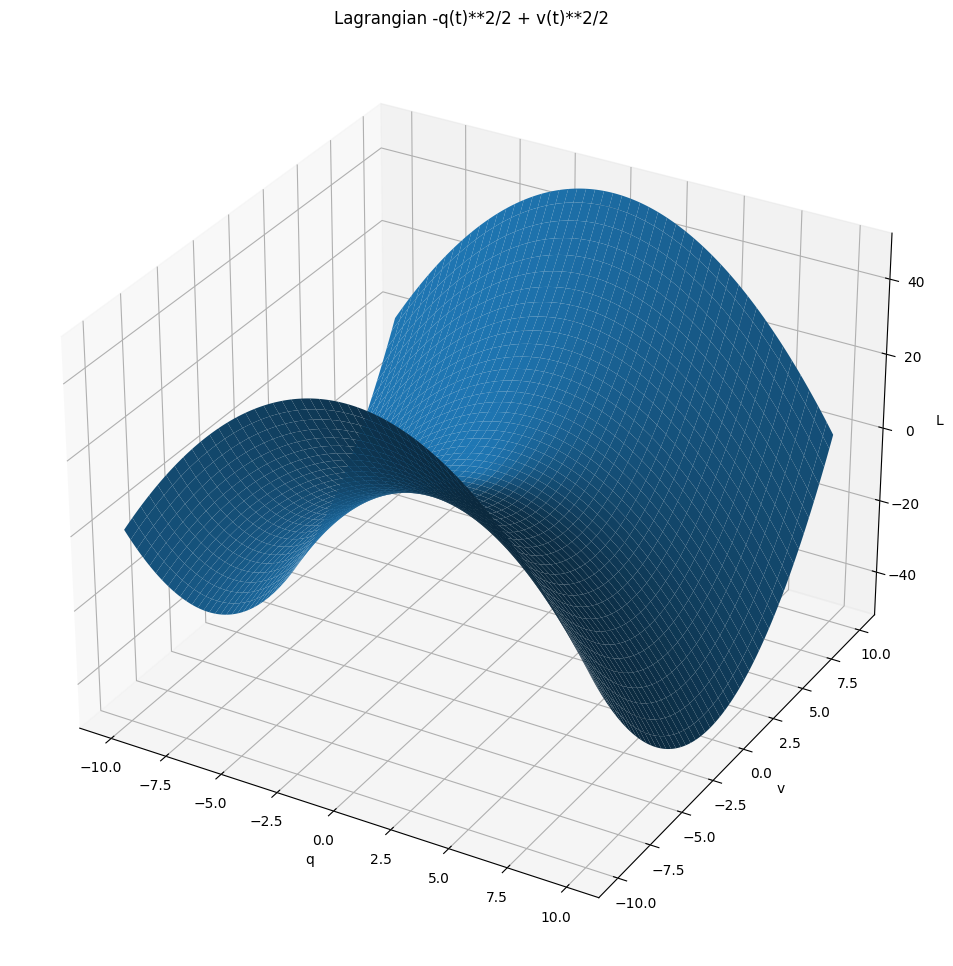
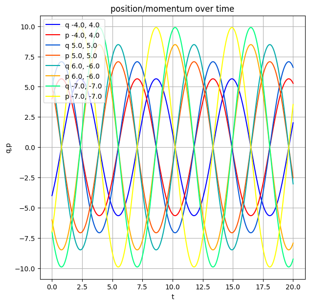
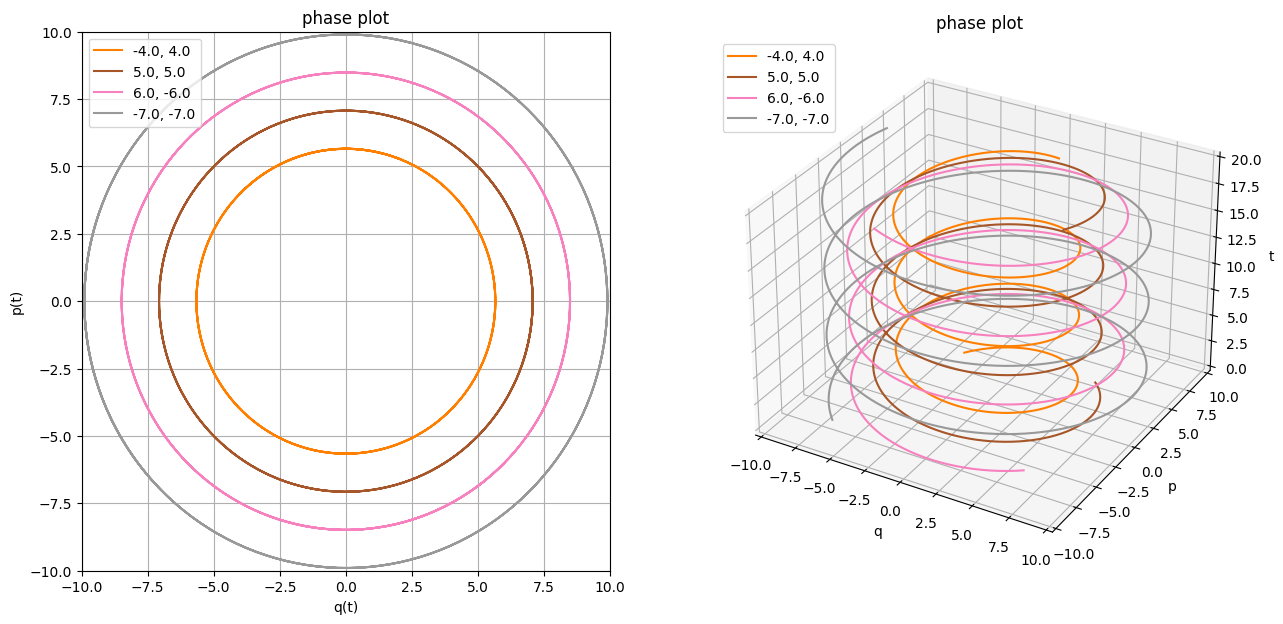
As expected, we get circular motion in the position-momentum plane and a nice spiral on the projective plot.

Let's try something else! TODO elaborate what it is -- it's like a potential hill? TODO use x instead of q?

In [7]:

L_hill = Lagrangian(v ** 2 / 2 + q ** 2 / 2)

# TODO print equations of motion??
# TODO def show time -- otherwise it's unclear where the point starts and where it goes
# TODO interesting... p and q seem to converge?? (yep, because when t goes to inf, they both go to A e^t)
# TODO again, it's impossible to spot the minimizing trajectories
# 1. the variation: ????
# 2. but also it has to satisfy q' = v (and unclear how to see that easily on the surface?)
# e.g. q = e^t, v = e^t
# variation-wise, we can rotate both q and v in the q-v plane, because L is symmetric
# but that would violate q' = v??
plot_motion(
    L_hill, 
    q0p0s=[
        # TODO these are more interesting?
        #(-1, -4),
        #(1 , 4),
        #(1 , -1),
        #(-1, 1),
        #(-1, 2),
        (-1, -1),
        (1 ,  1),
        (1 , -1),
        (-1,  1),
    ],
    q_max=2,
    p_max=2,
    T_max=2,
)
# Ok, so p = A e^t and q = A e^t are solutions
# There is a rotational symmetry for this lagrangian?? does this mean anything for the solutions?
# e.g. what if we rotate both p and q by a certain angle?
# will this break p = q' condition (or whatever their relation is???)
# E.g. we could rotate into q = 0, but that wouldn't make sense for p? uhh..
# TODO rename to 'phase portrait'

$L$ = $\frac{q^{2}{\left(t \right)}}{2} + \frac{v^{2}{\left(t \right)}}{2}$

$p$ over $v$: $p{\left(t \right)} = v{\left(t \right)}$

$v$ over $p$: $v{\left(t \right)} = p{\left(t \right)}$

$H$ = $\frac{p^{2}{\left(t \right)}}{2} - \frac{q^{2}{\left(t \right)}}{2}$

Hamilton's equations: $\left[ \frac{d}{d t} q{\left(t \right)} = p{\left(t \right)}, \ \frac{d}{d t} p{\left(t \right)} = q{\left(t \right)}\right]$

{'no_of_equation': 2, 'eq': [-p(t) + Derivative(q(t), t), -q(t) + Derivative(p(t), t)], 'func': [q(t), p(t)], 'order': {p(t): 1, q(t): 1}, 'func_coeff': {(0, q(t), 0): 0, (0, q(t), 1): 1, (0, p(t), 0): -1, (0, p(t), 1): 0, (1, q(t), 0): -1, (1, q(t), 1): 0, (1, p(t), 0): 0, (1, p(t), 1): 1}, 'is_linear': True, 'type_of_equation': None}

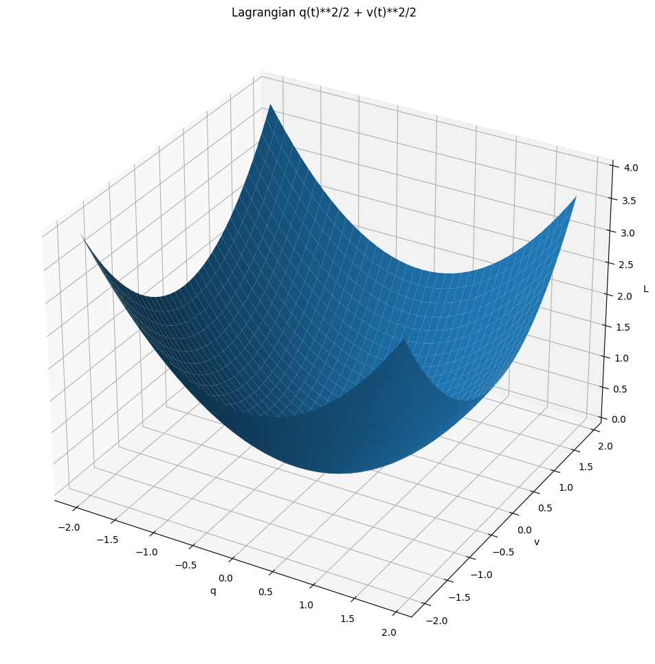
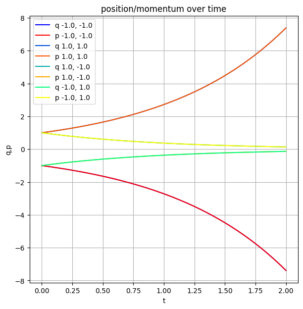
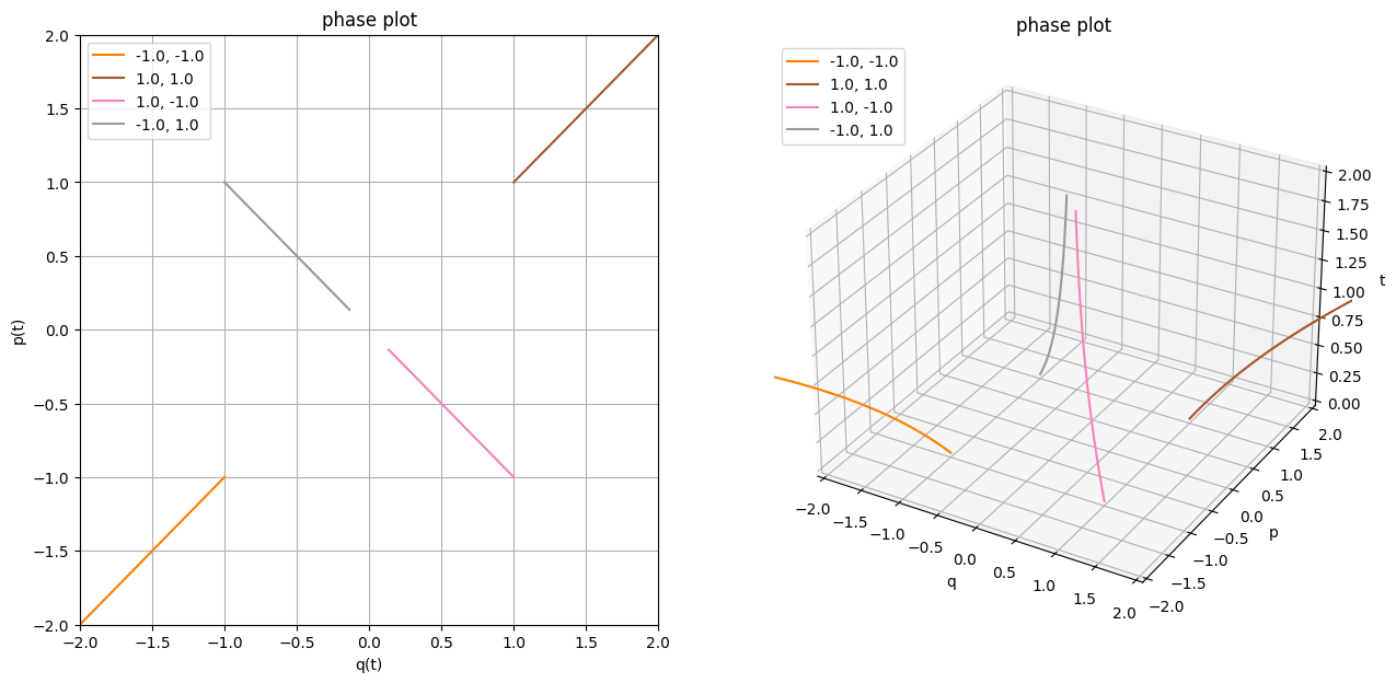
If you think about it, here we've got a potential hill! So the only equilibrium for this system is $q=0, p=0$. (TODO principle of least action?) Within this Lagrangian, you can reach it if your momentum (which coincides (TODO bad word) with velocity) is larger than the position in absolute value and of the opposite sign.

If the sign you your momentum is same as the sign of your position, you're basically forever doomed to slide down the potential! We can illustrate that by plotting more phase plots:

In [8]:

def circle(R, phis):
    return [(R * sin(phi), R * cos(phi)) for phi in phis]

def circlespace(R, points):
    return circle(R, linspace(0, 2 * np.pi, points))

plot_motion(
    L_hill,
    q0p0s=circlespace(R=5.0, points=36),
    T_max=3,
    p_max=5, q_max=5,
    plot_lag=False, plot_pq=False, plot_legends=False,
)

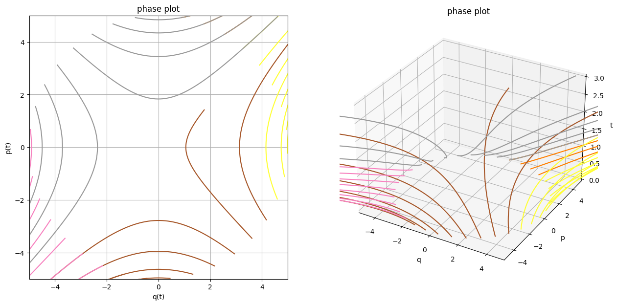
If you look at the 2D phase plot, you can clearly spot hyperbolas. This is not a coincidence considering that the Hamiltonian can be interpreted as energy which is conserved during the motion, and the lines where $p^2 + q^2 = \text{const}$ are precisely hyperbolas!

Actually, matplotlib allows us to plot something even nicer: quiver (usually called vector field or slope field) and streamplot.

In [9]:

def plot_ham_field(
    lagrangian, 
    steps=30, 
    qlim=None, 
    plim=None,
    density=1,
):
    dq, dp = lagrangian.dq_dp
    
    qs = linspace(*qlim, steps)
    ps = linspace(*plim, steps)
    Q, P = np.meshgrid(qs, ps)
    
    T = 0 # we're exploiting knowledge that hamiltonians are time independent in our case
    Hq = dq(Q, P, T)
    Hp = dp(Q, P, T)
    
    fig, ax = plt.subplots()
    ax.set_title("Hamiltonian vector field")
    ax.set_xlabel('q')
    ax.set_ylabel('p')
    ax.set_aspect(aspect=1)
    ax.streamplot(qs, ps, Hq, Hp, arrowstyle='-', density=density)
    ax.quiver(qs, ps, Hq, Hp, scale=100)
    plt.show()

In [10]:

# TODO rename _ham_; remove plot_ prefile?, rename qlim/plim?
plot_ham_field(L_hill, qlim=(-7, 7), plim=(-7, 7))
# TODO animation would be nice? sort of like bunch of particles of different color, flowing through space?

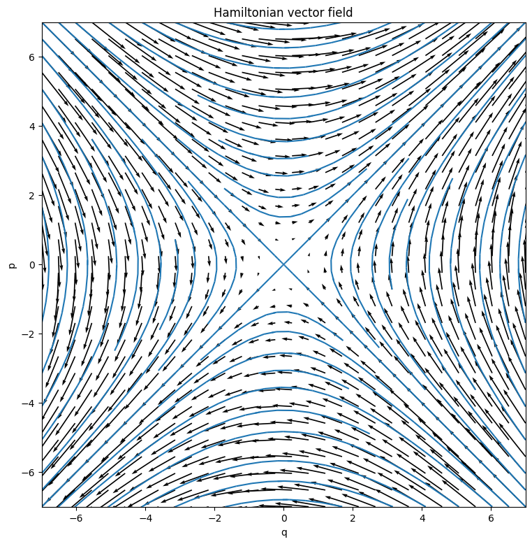
In this form it's easier to interpret this vector field physically: if you put a particle somewhere, it would follow the arrows. In this case as you can see, particles shoot off at infinity no matter what, which makes it evident why is that Lagrangian unpphysical (although doesn't explain what is it in the shape of Lagrangian that makes it so).

Grant Sanderson (3Blue1Brown) has a nice video featuring some animated vector field flows.

Ok, now let's try something truly weird.

In [11]:

L = Lagrangian(1 / 2 * v ** 2 * q ** 2)

# TODO L = half * v ** 2 * q
# TODO hmmm. I used to have q^2. Can it be problematic for legendre transform?? Seems ok in terms of having inverse though
# TODO investigate it separately?? 
# TODO analytical solution https://www.wolframalpha.com/input/?i=q%27%3Dp%2Fq;+p%27%3Dp%5E2%2F+(2+*+q%5E2)
# doesn't seem to behave well for negative time. something has to be wrong, right?)

# TODO ok, if we set T_max to 0.5, we get warnings that are impossible to get rid of..
# presumably from sysode?
# from IPython.utils import io
# with io.capture_output(display=False) as captured: -- doesn't work :(
# https://stackoverflow.com/a/22434262/706389 -- doesn't work either, ipython intercepts fd 0?

plot_motion(
    L, 
    q0p0s=[
        (-1, -1),
        (1 , 1),
        (1 , -1),
        (-1, 1),
    ],
    q_max=2,
    p_max=2,
    T_max=0.48,
)

$L$ = $0.5 q^{2}{\left(t \right)} v^{2}{\left(t \right)}$

$p$ over $v$: $p{\left(t \right)} = 1.0 q^{2}{\left(t \right)} v{\left(t \right)}$

$v$ over $p$: $v{\left(t \right)} = \frac{p{\left(t \right)}}{q^{2}{\left(t \right)}}$

$H$ = $\frac{0.5 p^{2}{\left(t \right)}}{q^{2}{\left(t \right)}}$

Hamilton's equations: $\left[ \frac{d}{d t} q{\left(t \right)} = \frac{1.0 p{\left(t \right)}}{q^{2}{\left(t \right)}}, \ \frac{d}{d t} p{\left(t \right)} = \frac{1.0 p^{2}{\left(t \right)}}{q^{3}{\left(t \right)}}\right]$

{'no_of_equation': 2, 'eq': [-1.0*p(t)/q(t)**2 + Derivative(q(t), t), -1.0*p(t)**2/q(t)**3 + Derivative(p(t), t)], 'func': [q(t), p(t)], 'order': {p(t): 1, q(t): 1}, 'func_coeff': {(0, q(t), 0): 0, (0, q(t), 1): 1, (0, p(t), 0): -1.0/q(t)**2, (0, p(t), 1): 0, (1, q(t), 0): 0, (1, q(t), 1): 0, (1, p(t), 0): 0, (1, p(t), 1): 1}, 'is_linear': False, 'type_of_equation': 'type3'}

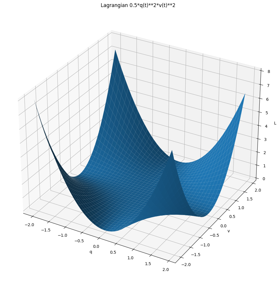
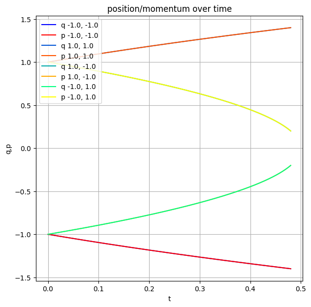
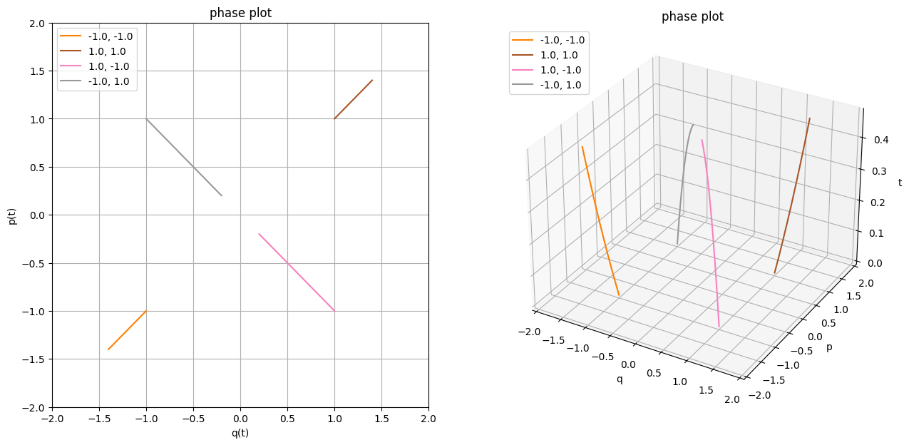
Now this is something fun! We get some warning from the ODE solver. I've cheated a bit and chosen T_max carefully here, if you increase it past 0.5, the numerical solution just goes nuts. And fair enough, if you look at the Hamiltonian, when $q=0$ clearly something bad has to happen. Sadly, Sympy got a bug in the solver for that type of equations, so let's try doing it the old, manual way.

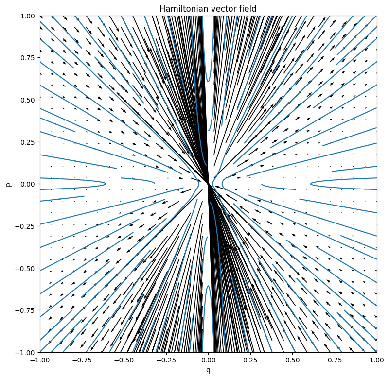
Starting with $\left [ \frac{d}{d t} q{\left (t \right )} = \frac{p{\left (t \right )}}{q^{2}{\left (t \right )}}, \quad \frac{d}{d t} p{\left (t \right )} = \frac{p^{2}{\left (t \right )}}{q^{3}{\left (t \right )}}\right ]$, if we divide LH and RH sides, we get something nice: (TODO ugh, not sure if we can do that formally... perhaps express second equation over p(t) from first...)

$$\frac{q'(t)}{p'(t)} = \frac{q(t)}{p(t)}$$$$\frac{q'(t)}{q(t)} = \frac{p'(t)}{p(t)}$$

If we integrate both parts, we get $$\ln q(t) = \ln p(t) + C$$ or, equivalently, $$q(t) = C p(t)$$

I find it interesting that we kind of could have seen it coming from the Hamiltonian if we think about what does it take for it to be a constant along the trajectory. Not sure if this argument can be generally useful though. But the important bit is that in our case, we have $H = \frac{1}{2 C^2}$, so surely there can't be problem when $q = 0$. Let's dig further. If we substitute or result for $q$ in its Hamiltonian equation, we get:

$$C p'(t) = \frac{p(t)}{C^2 p^2(t)}$$$$ p'(t) = \frac{1}{C^2} \frac{1}{p(t)}$$$$p^2(t) = \frac{1}{C^2} t^2 + D$$

TODO ugh. fucking hell, I'm stuck. Say we fixed p(0) = 1, q(0) = -1. Then, C = -1; D = 1 and p^2 = t^2 + 1. That means that p(t) is a parabola with minimum at t = 0 right? However judging by the vector field it would end up at 0 at some point. what am I missing??? have I lost the coupling somehow? pretty sure that isn't solvable explicitly and I just made a mistake somewhere.. TODO hmm. Unless it takes infinite time to get from t = 0?? probably bullshit though...

fucking hell, I'm so tired of this. also somthing in 'simpler equation.ipynb' q'=p/q; p'=q/p http://www.maths.surrey.ac.uk/explore/vithyaspages/coupled.html

First thing that I find interesting is that this clearly discriminates against negative $t$. TODO is that interesting actually?

Second, is that it's easy to see that when

TODO ugh, must have something to do with branch cuts...

TODO shit. maybe just give up on this one and write something about non-regularity (as in, lagrangian is non-regular over the whole q = 0 line)

It's hard to tell what this Lagrangian represents TODO let me know. TODO highligh todos in hakyll/ci? TODO wtf?? slope field in wolfram is complete https://www.wolframalpha.com/input/?i=q%27%3Dp%2Fq%5E2;+p%27%3Dp%5E2%2Fq%5E3 TODO mm. does it depend on which solution you choose or what? TODO huh? wolfram is solving it in complex numbers... https://www.wolframalpha.com/input/?i=q%27%3Dp%2Fq%5E2;+p%27%3Dp%5E2%2Fq%5E3+,+q(0)%3D-5,+p(0)%3D5

TODO investigate what happens around 0...

In [12]:

plot_ham_field(L, qlim=(-1, 1), plim=(-1, 1))

Let's try something else

In [13]:

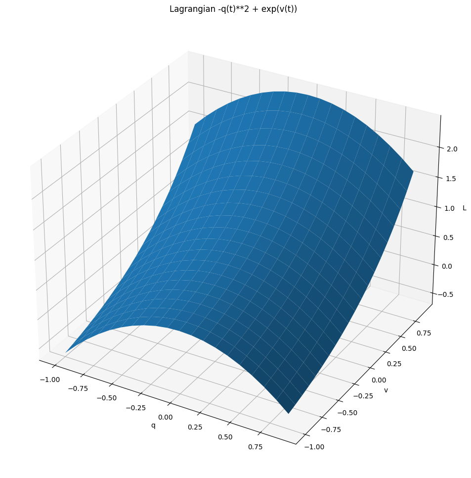
L = Lagrangian(exp(v) - q ** 2)
plot_motion(
    L, 
    q0p0s=[
        (-1, -1),
        (1 , 1),
        (1 , -1),
        (-1, 1),
    ],
    T_max=0.5,
    p_max=1,
    q_max=1,
    plot_phase=False,
)

$L$ = $- q^{2}{\left(t \right)} + e^{v{\left(t \right)}}$

$p$ over $v$: $p{\left(t \right)} = e^{v{\left(t \right)}}$

$v$ over $p$: $v{\left(t \right)} = \log{\left(p{\left(t \right)} \right)}$

$H$ = $p{\left(t \right)} \log{\left(p{\left(t \right)} \right)} - p{\left(t \right)} + q^{2}{\left(t \right)}$

Hamilton's equations: $\left[ \frac{d}{d t} q{\left(t \right)} = \log{\left(p{\left(t \right)} \right)}, \ \frac{d}{d t} p{\left(t \right)} = - 2 q{\left(t \right)}\right]$

{'no_of_equation': 2, 'eq': [-log(p(t)) + Derivative(q(t), t), 2*q(t) + Derivative(p(t), t)], 'func': [q(t), p(t)], 'order': {p(t): 1, q(t): 1}, 'func_coeff': {(0, q(t), 0): 0, (0, q(t), 1): 1, (0, p(t), 0): 0, (0, p(t), 1): 0, (1, q(t), 0): 2, (1, q(t), 1): 0, (1, p(t), 0): 0, (1, p(t), 1): 1}, 'is_linear': False, 'type_of_equation': 'type3'}

<lambdifygenerated-10>:2: RuntimeWarning: invalid value encountered in log
  return (log(_Dummy_132))

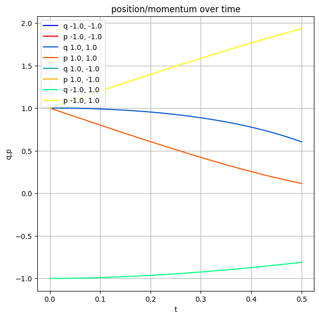
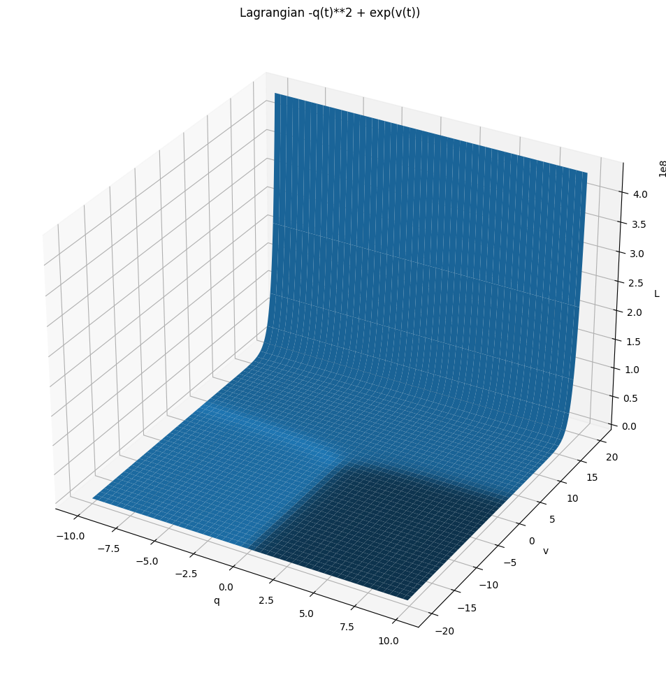
Uh-oh, momentum appears under logarigthm. Let's just exclude negative momentum for now..

In [14]:

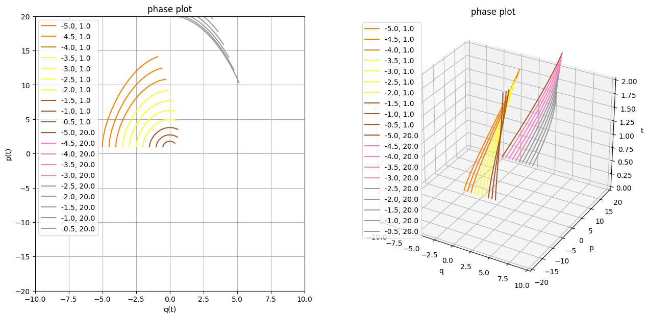
plot_motion(
    L, 
    q0p0s=[(q0, 1) for q0 in np.linspace(-5, -0.5, 10)] + [(q0, 20) for q0 in np.linspace(-5, -0.5, 10)],
    T_max=2,
    p_max=20,
    q_max=10,
    plot_pq=False,
)
plot_ham_field(
    L, 
    qlim=(-5, 5), plim=(0, 5),
    density=2,
)

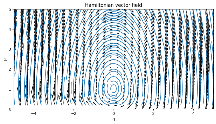
<lambdifygenerated-10>:2: RuntimeWarning: divide by zero encountered in log
  return (log(_Dummy_132))

TODO interesting! look at slope field, this lagrangian is always doomed!!! TODO what if we continue it to complex plane? TODO hmm. is the initial position the only thing defining when it dies?? TODO nah, se below, it seems pretty random.. TODO what happens to energy here?? Yep, exactly. when the energy is positive, it's fucked! TODO figure out how this relates? TODO it's a funny universe TODO huh, x log x is 0 when x -> 0 basically, we need to find when slope of the phase plot is 0? so p'(t) = 0

It's interesting though that the flow begs for continuation past the $p = 0$ line. Quick speculation: if you take your momentum as purely complex, you can draw in TODO draw. Not sure if it has any interesting physical, mathematical consequences, so I guess I'll have to look at it some other time (leave visible TODO?).

Let's take a closer look at the stable phase orbits. TODO time flow?

In [15]:

plot_motion(
    L, 
    q0p0s=[(-0.2, p0) for p0 in np.linspace(1.0, 2.67, 15)],
    T_max=30,
    plot_lag=False, plot_pq=False,
)

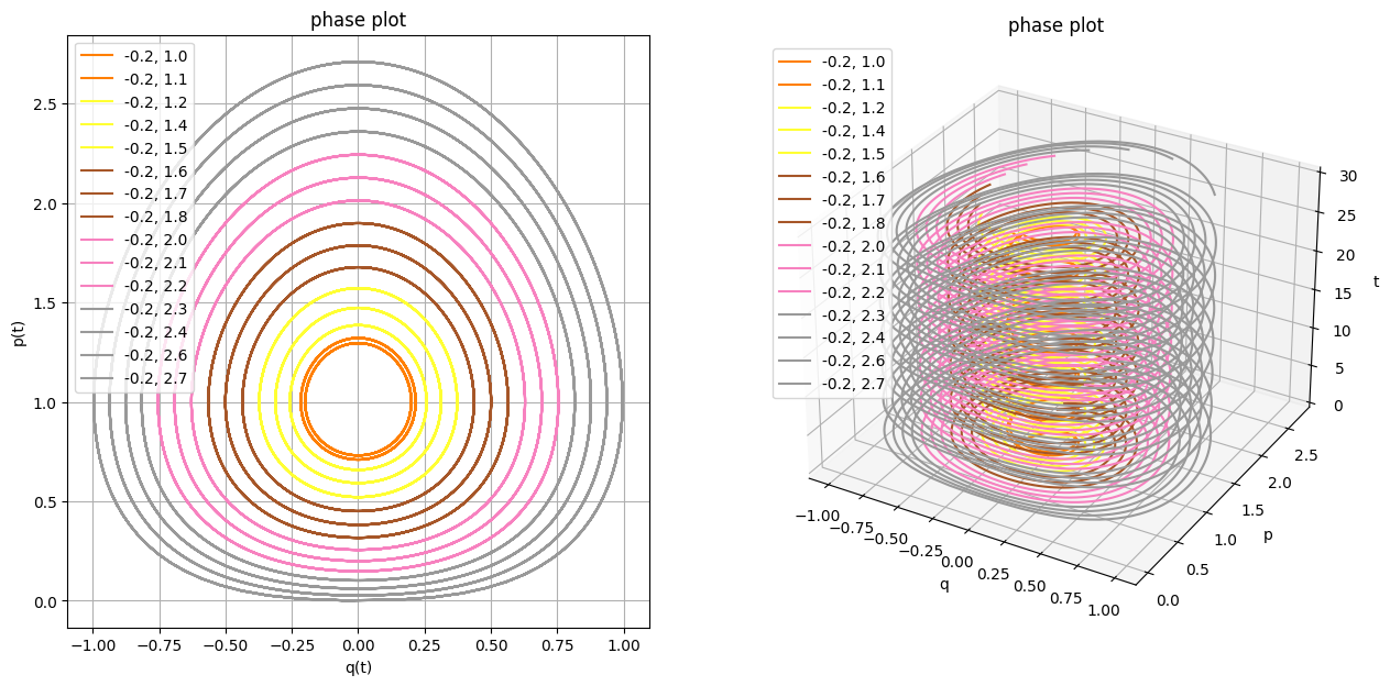
TODO hmm. interesting that all orbits seem to evolve at the same rate? why is that? definitely need animation...

TODO generate table of contents from tags or something?

TODO summarise what's hard to do. also smth about lagrangians

TODO maybe move it to the end? It also involved lots of yak shaving:

TODO sage/sympy
TODO finding out about symplectic integration
TODO figuring out literate programming in ipython notebooks TODO share hacks later
TODO fighting with emacs in order to render output the way I want it to

This post assumes some prior knowledge of TODO

TODO yak shaving TODO I wanted to figure out what does

spoiler: something called 'regularity', but I still have to figure that out so hopefully will write about it some other time

TODO what I don't like: It's very hard to 'evolve' code over time to let the reader follow your thoughts best you can do is copy paste, but that doesn't give you good perhaps that could be solved if you keep individual functions under git and reference the revisions or something like that, then you would get diffs for free. or google-wave like evolution of the whole notebook? However that would be hard to TODO

(you can see that I've defined huge chunks of code in advance)